
Learn
Steinhart-Hart Calculator
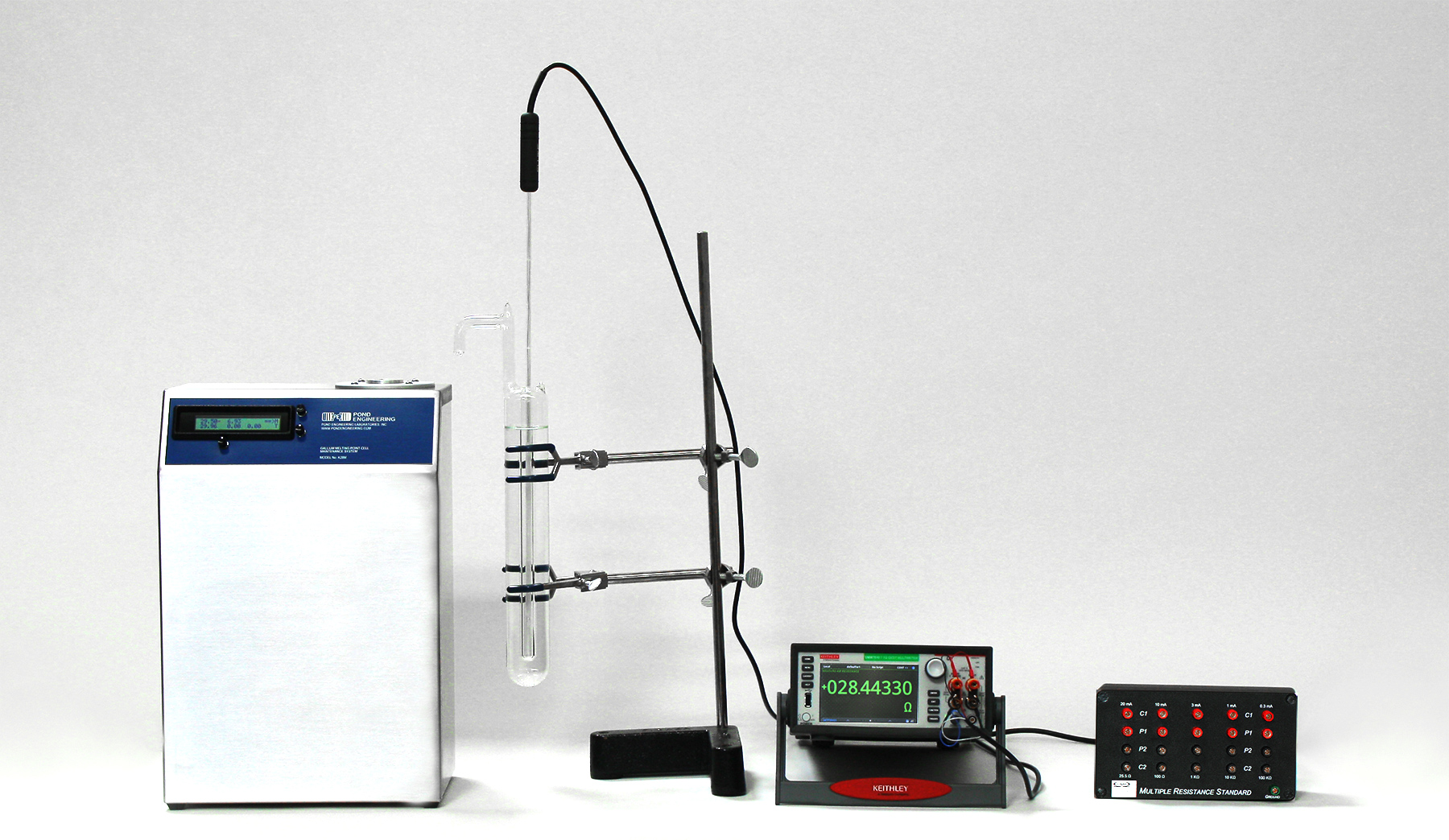
Convert NTC thermistor resistance to temperature with Steinhart-Hart coefficients, or fit your own 3-, 4-, or 5-term coefficients from calibration data — and see the linear algebra behind the calculation.
Interactive calculator
1/T = A + B·ln(R/R₀) + C·ln(R/R₀)² + D·ln(R/R₀)³
T is in kelvin, logarithms are natural, and R is in ohms. R₀ is the reference resistance the coefficients are defined against — the defaults here use R₀ = R25 = 10000 Ω. Set R₀ = 1 for coefficient sets specified directly on ln(R), which is how most published sets are written.
Coefficients accept scientific notation, for example 2.811578e-4.
Temperature
—
——
NTC (α) at this point—
NTC (α) at 25 °C—
R at 25 °C—
β25/85 (two-point)—
Resistance–temperature tableGenerated from the coefficients and R₀ above · −40 °C to 150 °C
| Temperature (°C) | Resistance (Ω) | NTC α (%/°C) | β at T (K) |
|---|
β at T is the local value at each temperature — the slope of the curve at that point. It is not the two-point datasheet spec β25/85, which is shown with the 25 °C results.
Temperature (°C)Resistance (Ω)Residual (mK)NTC (%/°C)Remove point
Fitted coefficients
NTC (α) AT 25 °C—
R at 25 °C from this fit: —
β25/85 (two-point) from this fit: —
25 °C is outside the calibration span — these values are extrapolated.
Resistance–temperature tableGenerated from the fitted coefficients · −40 °C to 150 °C
| Temperature (°C) | Resistance (Ω) | NTC α (%/°C) | β at T (K) |
|---|
β at T is the local value at each temperature — the slope of the curve at that point. It is not the two-point datasheet spec β25/85, which is shown with the fitted results above.
——
The Steinhart-Hart Equation
The Steinhart-Hart equation, published in 1968 by John Steinhart and Stanley Hart for oceanographic thermistor measurements, models the resistance vs. temperature characteristic of an NTC thermistor as a polynomial in the natural logarithm of resistance. The classic 3-term form is:
The 4-term form, which North Star Sensors prefers for wider temperature spans, restores the squared term:
Where T is the temperature in kelvin (°C + 273.15), R is the zero-power resistance in ohms, ln is the natural logarithm, and A, B, C, D are curve-fitting coefficients.
For the widest temperature spans, the series can be carried one term further, adding a fifth coefficient on the fourth power of the logarithm:
Interpolation error drops with every term added, and metrology laboratories use up to five terms for millikelvin-level work over wide ranges. Five-term fitting is uncommon among online thermistor calculators. One caution that comes with the fifth term: the fit becomes numerically delicate, so two programs may report visibly different A–E sets that nevertheless describe nearly the same curve over the calibrated span. Compare 5-term fits by the temperatures they produce, not by the individual coefficient digits, and always use a full set together.
The equation has a property that makes it especially practical: it is linear in the coefficients. Calculating temperature from resistance is a direct evaluation, and calculating coefficients from calibration data is a small linear-algebra problem — no iterative curve fitting required. The calculator above does both, and the sections below show how to reproduce it in a spreadsheet or in code.
Which Powers of ln(R) Belong in the Equation?
Looking at the classic form, it is natural to read the exponents {0, 1, 3} as a pattern — “odd powers only” — and to assume that a 4-term version should continue it with a fifth-power term, {0, 1, 3, 5}, rather than restore the square. The published record says otherwise, and the history is worth knowing.
In the original 1968 paper, Steinhart and Hart truncated the general series at the cubic and reported that including the squared term did not improve their fits, so they dropped it. A. S. Bennett re-examined that work in 1972 and showed the conclusion rested on a numerical error. The international metrology community’s reference document, the BIPM’s CCT Guide on Secondary Thermometry: Thermistor Thermometry, is direct about it: “the original recommendation for the equation was based on a numerical error,” the classic form “is only sometimes better than the normal 3-term equation” using {0, 1, 2}, and “the four-term version” — with consecutive powers {0, 1, 2, 3} — “is always more accurate” than the classic skip-the-square form. Broader comparisons of candidate calibration equations (Chen, 2009) have investigated the same family of thermistor calibration equations, and an approximation-theory analysis of thermistor calibration (White, 2017) shows interpolation error is governed by the temperature span and the number of fitted terms — adding the next consecutive term helps more than skipping ahead to a higher power.
There is also no metrology or material-symmetry reason to omit even powers. The NTC ceramic physics is commonly approximated by an activation law, R ≈ R∞·exp(β(T)/T), with β varying smoothly with temperature. A smooth inverse relationship between 1/T and ln(R) generally admits consecutive powers of ln(R), so even terms are not forbidden. The skipped square term in the classic Steinhart-Hart equation is best understood as a historical convention traceable to the numerical error discussed by Bennett and summarized in the BIPM thermistor guide, not as a property of the ceramic.
The practical guidance is therefore:
- The classic 3-term equation {0, 1, 3} is deeply established, is how most published coefficient sets are specified, and performs well over moderate spans. There is nothing wrong with using it where its accuracy is sufficient.
- When four coefficients are justified, use consecutive powers {0, 1, 2, 3} — not {0, 1, 3, 5}. This is the 4-term equation North Star Sensors uses for its published resistance vs. temperature tables.
- If still more accuracy is needed, the correct extension is the next consecutive term, {0, 1, 2, 3, 4} — available as the 5-term option in the calculator above — or a narrower calibration span; see the span guidelines on our Calculating Temperature from Resistance page.
How the Coefficient Fit Works
Fitting coefficients is solving a linear system. For each calibration point, measure the zero-power resistance R at a known temperature, convert the temperature to kelvin, and form y = 1/T and L = ln(R). Each point then gives one row of a matrix equation. For the 4-term equation with four calibration points:
With exactly as many points as coefficients, the solution is a = M⁻¹y — the fitted curve passes exactly through every calibration point. With more points than coefficients, the least-squares solution a = (MᵀM)⁻¹Mᵀy minimizes the sum of squared errors and averages out measurement noise; spreadsheet and numerical libraries solve this form directly. For the 3-term equation, drop the squared column and the matrix is 3 × 3; for the 5-term equation, add an L⁴ column and a fifth calibration point for a 5 × 5 system.
Because the equation gives 1/T as a function of ln(R), its derivative also yields the slope values used to specify thermistors. The local (tangent) Beta at any operating point is:
shown here for the 4-term form, and the NTC (alpha) follows directly from it:
with α multiplied by 100 to express it in % / °C. This local β is the slope of the curve at a single temperature — related to, but not the same as, a two-point specification such as β25/85, which is the average slope between two fixed temperatures: β25/85 = ln(R25/R85) / (1/T25 − 1/T85). The calculator reports the NTC and the two-point β25/85 alongside every result, includes α and local-β columns in its resistance–temperature tables, and in fitting mode evaluates the NTC at each of your calibration temperatures.
The NTC at 25 °C deserves special attention: North Star Sensors uses it to characterize an R/T curve material in its part numbering, where curve 44 means an NTC of approximately -4.4 % / °C. Evaluating the curve at exactly 25 °C runs the equation in reverse, which means solving numerically for ln(R) at 298.15 K; the calculator does this with a few Newton iterations and highlights the resulting NTC at 25 °C and R25 with every coefficient fit.
Doing It in a Spreadsheet
- Lay out one row per calibration point with columns for temperature
tin °C,T = t + 273.15,y = 1/T, andL = LN(R), then add columns forL^2andL^3(skipL^2for the 3-term equation, addL^4for the 5-term equation). - Build the matrix
M: a column of 1s followed by theL,L^2,L^3columns. - With exactly as many points as coefficients, select a vertical run of output cells and enter
=MMULT(MINVERSE(M), Y)as an array formula, whereYis the1/Tcolumn. The result isA,B,C,Dfrom top to bottom. - With more points than coefficients,
=LINEST(Y, Lcols)returns the least-squares coefficients in one step — note that LINEST lists them in reverse order, highest power first. - To convert a resistance to temperature:
=1/(A + B*LN(R) + C*LN(R)^2 + D*LN(R)^3) - 273.15.
This is exactly the method in our downloadable Steinhart-Hart Coefficients Calculator spreadsheet, which applies the 4-point matrix solution to North Star Sensors’ standard curves.
Doing It in Code
Any language with a least-squares routine can do the fit in a few lines. In Python with NumPy:
import numpy as np

t_c = np.array([0.00, 16.67, 33.33, 50.00])           # calibration temperatures, deg C
r_ohm = np.array([30196.0, 14149.0, 7202.0, 3929.0])  # measured resistances, ohms

y = 1.0 / (t_c + 273.15)   # 1/T in 1/K
L = np.log(r_ohm)          # natural log of resistance

M = np.column_stack([L**0, L**1, L**2, L**3])  # 3-term: [L**0, L**1, L**3] — 5-term: append L**4
A, B, C, D = np.linalg.lstsq(M, y, rcond=None)[0]

def temperature_c(r):
    Lr = np.log(r)
    return 1.0 / (A + B*Lr + C*Lr**2 + D*Lr**3) - 273.15
np.linalg.lstsq handles the exact 4-point case and the overdetermined least-squares case with the same call. Evaluating temperature on a microcontroller needs only log() and a few multiplies — see our worked example in Temperature from a Thermistor: Arduino Code.
Practical Notes
- Work in kelvin inside the equation and convert to °C only at the end. Mixing units is the most common source of wildly wrong results.
- Use the natural logarithm (
LNin Excel,login Python and C) — not the base-10 logarithm. - Coefficients are tied to the units and convention used to fit them. A set fitted with
Rin ohms differs from a set fitted withRin kilohms or with a resistance ratio such asln(R/R25); always carry the convention along with the values. The calculator’sR₀field handles ratio-based coefficient sets. - Choose calibration points that span the temperature range your application actually uses, spaced roughly evenly, and avoid using the fitted curve outside that range — interpolation error grows very quickly under extrapolation.
- Adding a few extra calibration points beyond the minimum and letting least squares average them is a simple way to reduce sensitivity to measurement noise in any single point.
- Interpolation error depends strongly on the temperature span. For span-by-span accuracy guidelines and how North Star Sensors builds its published R/T tables, see Calculating Temperature from Resistance.
Why does the curve look like this? Inside the Lattice — an interactive look at the physics behind the equation